1.2 The Periodic Table

The periodic table also offers a lot of information geologists use! Understanding why elements in the periodic table are arranged in a particular way helps us understand major geological concepts better.

The arrangement of elements in the periodic table based on their physical and chemical properties is arguably one of the most outstanding scientific achievements. Over hundreds of years, scientists have studied elemental properties and how to organize them. It culminated in the work of Dmitri Mendeleev (Dmitri Mendeleev - Wikipedia) - who finally created a version of the periodic table organized by atomic numbers of elements and arranged in groups and periods. This modern periodic table is arguably one of the greatest achievements in modern science.

Solving the puzzle of the periodic table - Eric Rosado | TED-Ed

The genius of Mendeleev’s periodic table | TED-Ed

Below is the latest version of the IUPAC periodic table. The International Union of Pure and Applied Chemistry (iupac.org) is a nonpolitical and international authority on chemical nomenclature and terminology, including the naming of new elements in the periodic table and all elemental data. This version supersedes all other versions of periodic tables in all your textbooks. The periodic table is updated when new elements are created, or new or updated data is available. Another good source of elemental information is Periodic Table - Ptable.

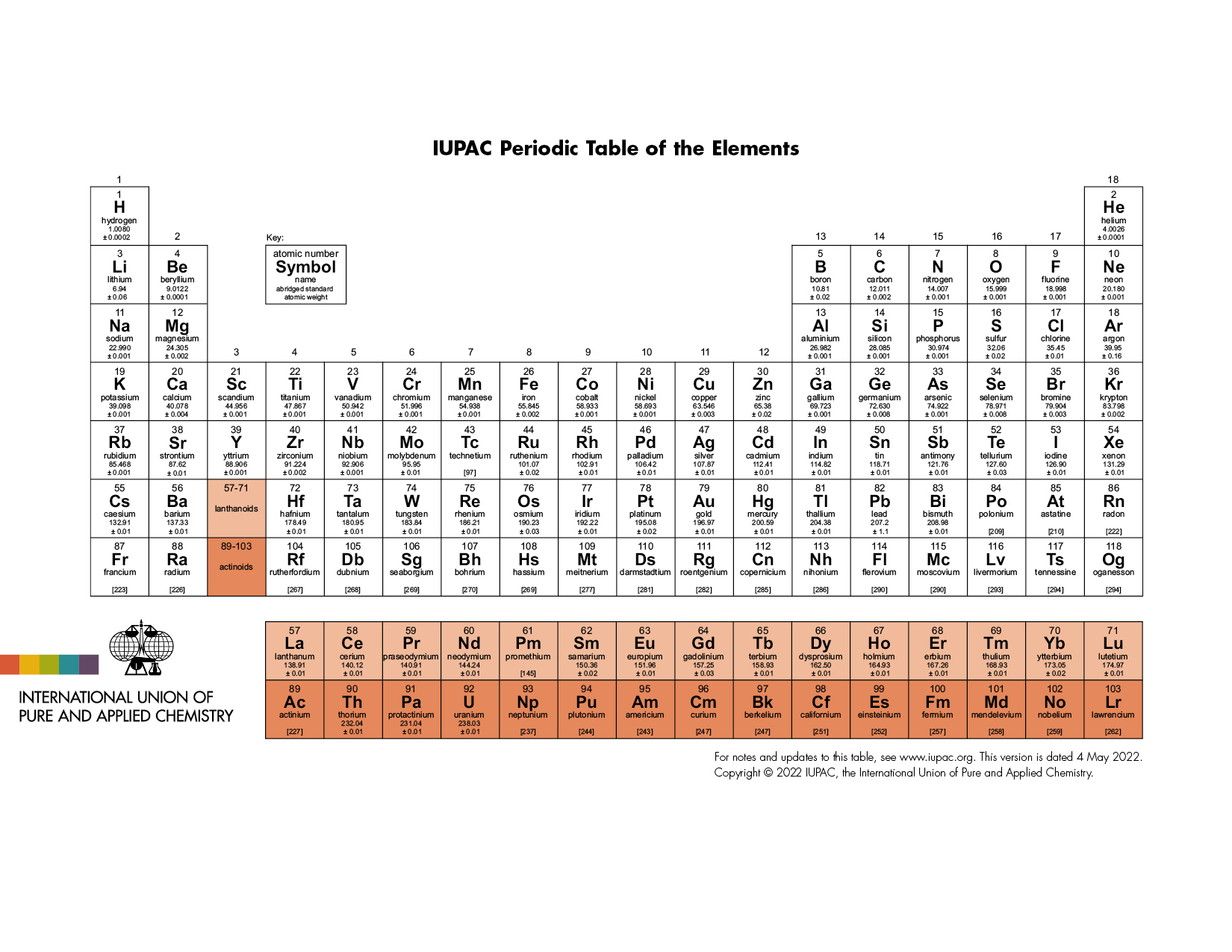
Fig. 4 The official IUPAC periodic table of elements. Image source: Periodic Table of Elements - IUPAC | International Union of Pure and Applied Chemistry

The element Md was named for Mendeleev. Most recently, elements 113, 115, 117, and 118 were named nihonium (Nh after Nihon or Japanese for the land of the rising sun), moscovium (Mc after a research lab in Moscow, Russia), tennessine (Ts in honor of research labs in Oak Ridge and Nashville, Tennessee), and oganesson (Og after Yuri Oganessian), respectively.

The periodic table contains 118 elements arranged according to the \(Z\) shown above each element. Except for \(\ce{H}\), nonmetals appear at the far right of the table. The two rows of metals below the main table are separated to keep the table from being too wide. The 1-18 group designation is an IUPAC recommendation.

The elements are arranged in periods, horizontal rows, in order of increasing \(Z\). The first period contains two elements, \(\ce{H}\) and \(\ce{He}\). The second and third periods contain eight elements: \(\ce{Li-Ne}\), and \(\ce{Na-Ar}\), respectively. The fourth and fifth periods contain 18 elements: \(\ce{K-Kr}\), and \(\ce{Rb-Xe}\), respectively.

Most elements can be categorized as metals or nonmetals. One of the properties that distinguishes metals from nonmetals is metals’ ability to conduct heat and/or electricity. Metalloids are elements with properties that are intermediate between those of metals and nonmetals. These include \(\ce{B, Si, Ge, As, Sb, Te, Po, and At}\). The figure below shows the main classes of elements in the periodic table.

Fig. 5 The periodic table organizes elements with similar properties into groups and periods. Image source: 3.6 The Periodic Table - Chemistry: Atoms First | OpenStax

Vertical columns in the periodic table are groups, referred to collectively by their group number (Group 1, Group 2, and so on). For convenience, some groups have special names: e.g., Group 1 are alkali metals, Group 2 are alkaline earth metals, Group 16 are chalcogens, Group 17 are halogens, and Group 18 are noble gases. Group 3-12 elements collectively are called the transition elements or the transition metals.

For more information, see 3.6 The Periodic Table - Chemistry: Atoms First | OpenStax.

Electron Configurations

Hydrogen’s atomic structure is the simplest of all elements due to the presence of just one electron in its atomic structure. For all other elements, quantum theory has to be applied to predict and describe the configuration of electrons in an atom. Due to their size and mass, subatomic particles are not governed by the same physical laws as all other substances on Earth.

Understanding the electronic structure of elements is fundamental to understanding how different minerals and rocks form. Further, knowledge of electron configurations helps us understand and predict the properties of the elements. It also explains why the elements fit into the periodic table the way they do.

Quantum Mechanics

Pioneering work in quantum theory (quantum, or the smallest quantity of energy emitted or absorbed, was proposed by German physicist Max Planck and later advanced by Einstein and others) revolutionized the whole field of physics and chemistry. Other ideas in quantum mechanics (e.g., Heisenberg uncertainty principle, Schrödinger’s equation) helped us understand the complex particle- and wave-like behavior of electrons around the nucleus.

Quantum mechanics does not allow us to specify the exact location of an electron in an atom, but it does define the region where the electron is most likely to be at a given time. Electron density gives the probability that an electron will be found in a particular region of an atom. In this description of an atom, we use atomic orbitals to refer to the wave function of an electron in an atom.

Quantum numbers are required to describe an atom’s electron density distribution. Each atomic orbital in an atom is characterized by a unique set of three quantum numbers: the principal quantum number (\(n\)), the angular momentum quantum number (\(l\)), and the magnetic quantum number (\(m_l\)).

The principal quantum number (\(n\)) designates the orbital size. Values of \(n\) are \(1,\ 2,\ 3,\ \ldots, \) etc. The larger the \(n\), the greater the distance of an electron in that orbital from the nucleus. A collection of orbitals with the same \(n\) value is called a shell.

The angular momentum quantum number (\(l\)) describes the shape of the orbital and depends on the value of \(n\) (range from 0 to \(n-1\)). One or more orbitals with the same \(n\) and \(l\) values are called subshells. E.g., \(2s\) and \(2p\). See Table 2 for orbital designations.

Table 2 Orbital designations

\(l\)	\(0\)	\(1\)	\(2\)	\(3\)
Orbital designation	\(s\)	\(p\)	\(d\)	\(f\)

The magnetic quantum number (\(m_l\)) describes the orbital orientation in space. Within a subshell, \(m_l\) depend on the value of \(l\) and there are (\(2l+1\)) values of \(m_l\) from \(-l,\ldots, 0, \ldots, +l\).

Though three quantum numbers are sufficient to describe an atomic orbital, an electron spin quantum number (\(m_s\)) is necessary to describe an electron that occupies the orbital. Physicists determined that electrons have magnetic properties due to electrons spinning on their axes. The \(m_s\) value specifies two possible and opposite directions of spin as \(+\frac{1}{2}\) and \(-\frac{1}{2}\). Quantum numbers are summarized in Table 3.

Table 3 Summary of quantum numbers

Quantum number	Symbol	Values
Principal	\(n\)	\(1, 2, 3, \ldots, \infty\)
Angular Momentum	\(l\)	\(n-1, n-2, n-3, \ldots, 0\)
Magnetic	\(m_l\)	\(0, \pm1, \pm2, \ldots, \pm l\)
Electronic Spin	\(m_s\)	\(\pm\frac{1}{2}\)

An electron’s magnetic properties are the origin of electromagnetism. This property is used to identify elements using a mass spectrometer. For more information, see 2.3 Atomic Structure and Symbolism - Chemistry: Atoms First | OpenStax

Atomic Orbitals

Even though it is hard to describe atomic orbitals, they are assigned specific shapes to help understand the formation of chemical bonds and molecular geometry in Earth materials. These shapes represent probability distributions for the location of the electron. The Heisenberg uncertainty principle tells us that it is impossible to simultaneously measure the position and momentum of a particle. In this case, the position of an electron is only approximately known. Fig. 6 shows these approximate locations at any time.

Fig. 6 Balloon diagrams show electron densities in \(s\), \(p\), and \(d\) orbitals. Source: 3.5 Periodic Variations in Element Properties - Chemistry: Atoms First | OpenStax

Electron Configurations

The \(\ce{H}\) atom is a straightforward system because it contains only one electron, which may reside in the \(1s\) orbital (the ground state) or some higher-energy orbital (an excited state). With many-electron systems, we need to know the ground-state electron configuration – i.e., how the electrons are distributed in the various atomic orbitals. We need to know the relative energies of atomic orbitals in a many-electron system, which differ from those in a one-electron system such as \(\ce{H}\).

Note

The ground state for a many-electron atom is the one in which all the electrons occupy orbitals of the lowest possible energy.

Fig. 7 shows the general order or orbital energies in a many-electron atom. In contrast to the \(\ce{H}\) atom, many-electron systems depend on \(n\) and \(l\) values. The general order in which electrons fill can be summarized in Fig. 8.

Using Pauli exclusion principle, no two electrons in an atom can have the same four quantum numbers. Because each orbital corresponds to a unique set of the first three quantum numbers and the spin quantum number has only two possible values, two electrons with opposite spins may occupy a given orbital.

Fig. 7 Orbital energy levels in many-electron atoms. For a given value of \(n\), orbital energy increases with \(l\). \(s\), \(p\), \(d\), and \(f\) levels can hold 2, 6, 10, and 14 electrons, respectively. Source: 3.5 Periodic Variations in Element Properties - Chemistry: Atoms First | OpenStax

We can write electron configurations for elements based on the order of orbital energies and the Pauli exclusion principle. The Aufbau principle makes it possible to “build” the periodic table of the elements and determine their electron configurations in steps. Each step involves adding one proton to the nucleus and one electron to the appropriate atomic orbital. Through this process, we gain a detailed knowledge of the electron configurations of the elements. The Hund’s rule states that the most stable arrangement of electrons in orbitals of equal energy is the one in which the number of electrons with the same spin is maximized, which is finally used to round up all the rules for writing the electron configurations.

Fig. 8 A simple way to remember the order in which orbitals fill with electrons. The arrow leads through each subshell in the appropriate filling order for electron configurations. This chart is straightforward to construct. Make a column for all the \(s\) orbitals with each \(n\) shell on a separate row. Repeat for \(p\), \(d\), and \(f\). Be sure to only include orbitals allowed by the quantum numbers (no \(1p\) or \(2d\), and so forth). Finally, draw diagonal lines from top to bottom as shown. Source: 3.5 Periodic Variations in Element Properties - Chemistry: Atoms First | OpenStax

General rules for writing electron configurations

The following general rules for determining the electron configuration of an element in the ground state:

1. Electrons will reside in the available orbitals of the lowest possible energy. The overall energy of the atom is minimized.

2. Each orbital can accommodate a maximum of two electrons.

3. Electrons will not pair in degenerate (equal energy) orbitals if an empty orbital is available.

4. The electrons will first be added singly to each available orbital for each set of orbitals (\(s\), \(p\), \(d\), \(f\)). After all the orbitals in a set have a single set of a single electron, subsequent electrons can enter these orbitals if they have the opposite spin.

5. Atoms attain maximum stability when the available orbitals are completely-filled, half-filled, or empty.

6. Orbitals will fill in the order indicated shown in Fig. 8, which provides a simple way for you to remember the proper order.

Example: Writing electron configuration

Let’s write the electron configuration of a calcium (\(\ce{Ca}\)) atom (\(Z = 20\)) using the general rules given above.

Because \(Z = 20\), we know that a \(\ce{Ca}\) atom has 20 electrons. They will fill orbitals in the order designated in Fig. Fig. 8. Remember, each \(s\), \(p\), \(d\), and \(f\) levels can hold 2, 6, 10, and 14 electrons, respectively. Follow that order and start assigning electrons to each orbital until you account for 20 electrons.

Orbitals will fill in the following order: \(1s^2 2s^2 2p^6 3s^2 3p^6 4s^2\).

Electron Configuration and the Periodic Table

Noble gases (\(\ce{He}\)-\(\ce{Rn}\), group 18 in the periodic table) have all their orbitals filled. Electron configurations of all other elements (except \(\ce{H}\)) can be represented using the noble gas core, i.e., the noble gas that precedes each element is shown in brackets, followed by the electron configuration in the outermost occupied subshells.

Example: Compressed electron configuration

Write the electron configuration of a calcium (\(\ce{Ca}\)) atom (\(Z = 20\)) using the abbreviated form.

\(\ce{Ne}\) is the closest preceding element with the electron configuration: \(1s^2 2s^2 2p^6 3s^2 3p^6\).

\(\therefore \ce{Ca}\) would be \(\ce{Ne}\)[\(4s^2\)].

Fig. 9 shows the electron configuration of all the elements in the periodic table in terms of the noble gas core. As seen in this figure, the electron configuration in each group has the outermost electrons in common. These outermost electrons are called valence electrons. These valence electrons determine how atoms interact with one another. Having the same valence-electron configuration causes the elements in the same group to exhibit similar chemical properties. In the next section, we explore these trends in the periodic table.

Fig. 9 Electron configuration of elements in the periodic table using the noble gas core. Image Source: 3.4 Electronic Structure of Atoms (Electron Configurations) - Chemistry: Atoms First | OpenStax

Trends in the Periodic Table

Effective nuclear charge

Nuclear charge (\(Z\)) is the number of protons in the nucleus of an atom and influences how much of this positive charge electrons experience and is expressed as effective nuclear charge (\(Z_\textrm{eff}\)). Since H has only one electron, \(Z=Z_\textrm{eff}\), but this is not the case for the rest of the elements. In all other atoms, the electrons are simultaneously attracted to the nucleus and repelled by one another. An electron in a many-electron atom is partially shielded from the positive charge of the nucleus by the other electrons in the atom. If an electron is removed from an atom, the effective nuclear charge increases, and more energy is required to remove any subsequent electrons; therefore, \(Z_\textrm{eff}\) increases from left to right in each period of the periodic table. Similarly, \(Z_\textrm{eff}\) increases from top to bottom in each group as each step down a group represents a significant increase in \(Z\) and an additional shell of core electrons to shield the valence electrons from the nucleus. Several of the physical and chemical properties are dependent on \(Z_\textrm{eff}\).

Atomic Radius

We envision that atoms are spherical and intuit that the atomic radius of an atom is the distance between the nucleus and the valence shell. But, according to quantum mechanics, no specific distance an electron can be found beyond the nucleus. So we operationally define the atomic radius in two ways: (i) the metallic radius – half the distance between the nuclei of two adjacent, identical metal atoms and (ii) the covalent radius – half the distance between adjacent, identical nuclei that are connected by a chemical bond.

Fig. 10 Atomic radii trends in the periodic table. The units are in picometers (\(\pu{e-12 m}\). Image source: 3.5 Periodic Variations in Element Properties - Chemistry: Atoms First | OpenStax

As seen in Fig. 10 shows the electron configuration of all the elements in the periodic table, the atomic radius decreases as we move from left to right across a period and increases from top to bottom as we move down within a group. This trend may be counter-intuitive. Isn’t the atomic radius supposed to increase as we go from left to right in each period? In the previous section, we found that \(Z_{eff}\) increases from left to right in each period, i.e., there is powerful attraction between the nucleus and the valence shell when the magnitudes of both charges increase. Therefore, as we move from left to right in each period, the valence shell is drawn closer to the nucleus, making the atomic radius smaller. Within each period, the trend in atomic radius decreases as \(Z\) increases; for example, from \(\ce{K}\) to \(\ce{Kr}\). Within each group (e.g., the alkali metals shown in purple), the trend is that atomic radius increases as \(Z\) increases.

Fig. 11 The atomic radius decreases within each period as \(Z\) increases; for example, from \(\ce{K}\) to \(\ce{Kr}\). Within each group (e.g., the alkali metals shown in purple), the atomic radius increases as \(Z\) increases. Image source: 3.5 Periodic Variations in Element Properties - Chemistry: Atoms First | OpenStax

Ionic radius is related to atomic radius but is deduced from bond length when the atom is bonded to one or more other atoms. As seen in Fig. 12, cations have smaller ionic radii than do anions. Also, the ionic radius decreases as the charge increases. This decrease is due to the loss of outer electrons and the shrinking of the orbits of the remaining electrons. The latter occurs because fewer electrons share the charge of the nucleus and hence have a greater attractive force on each. In addition, the ionic radius increases downward in each group in the periodic table, both because of the addition of electrons to outer shells and because these outer electrons are increasingly shielded from the nuclear charge by the inner ones. Ionic radius is important in determining geochemical properties such as substitution in solids, solubility, and diffusion rates. Large ions need to be surrounded, or coordinated, by more oppositely charged ions than smaller ones.

Fig. 12 The radius for a cation is smaller than the parent atom (\(\ce{Al}\)), due to the lost electrons; the radius for an anion is larger than the parent (\(\ce{S}\)), due to the gained electrons. The values are in \(\pu{pm}\) (= \(\pu{e-12 m}\)). Image source: 3.5 Periodic Variations in Element Properties - Chemistry: Atoms First | OpenStax

Ionization Energy

Ionization energy (IE) is the minimum energy required to remove an electron from an atom in the gas phase, forming a cation (ion with a positive charge).

\[\ce{Na -> Na^+ + e^-}\]

The above reaction shows the ionization of \(\ce{Na}\) to \(\ce{Na^+}\), both in gas phases and the release of an electron (denoted as \(\ce{e^-}\)). The ionization energy is expressed in \(\pu{kJ mol-1}\) or the number of kilojoules required to remove a mole of electrons from a mole of gaseous atoms. In the above \(\ce{Na}\) ionization reaction, IE \(= \pu{495.8 kJ mol-1}\). Specifically, this is the first ionization energy of sodium, IE\(_1\) (Na), which corresponds to the removal of the most loosely held electron from each \(\ce{Na}\) atom. Fig. 13 shows IE\(_1\) of elements in the periodic table. In general, as the nuclear charge (\(Z_{eff}\)) increases, IE also increases.

Fig. 13 First ionization energy of elements. Image source: 3.5 Periodic Variations in Element Properties - Chemistry: Atoms First | OpenStax

It is possible to remove additional electrons from the atoms; however, removing each successive electron requires expending enormous amounts of energy. It is harder to remove an electron from a cation than from an atom (and it gets even more challenging as the charge on the cation increases). Since core electrons are closer to the nucleus, they experience strong \(Z_{eff}\). Additionally, fewer filled shells are shielding them from the nucleus.

Electron Affinity

Electron affinity (EA) is the energy released when an atom in the gas phase accepts an electron, forming an anion (ion with a negative charge).

\[\ce{Cl + e^- -> Cl^-}\]

In the above reaction, one mole of gaseous Cl accepts a mole of electrons, releasing \(\pu{349.0 kJ mol-1}\) of energy.

See Fig. 14 for EA trends in the main group elements in the periodic table. Like IE, EA increases from left to right across a period due to an increase in \(Z_{eff}\) from left to right. Adding negatively charged electrons to atoms becomes easier as the number of positively charged protons increases in the nucleus.

Fig. 14 Electron affinities of main group elements in the periodic table. Image source: 3.5 Periodic Variations in Element Properties - Chemistry: Atoms First | OpenStax

Electronegativity

Electronegativity quantifies the tendency of an element to attract shared electrons (in a covalent bond) to itself. It is a parameter used to characterize the behavior of the elements and is inversely correlated with atomic radii within each periodic table group. It determines how the electron density in a molecule or a polyatomic ion is distributed. An element with a high electronegativity tends to attract electron density more than an element with low electronegativity. Electronegativity is a relative concept and can be measured only relative to the electronegativity of other elements. Fig. 15 shows trends in the periodic table. We can qualitatively predict an atom’s electronegativity based on its EA and IE\(_1\). In general, electronegativity increases from left to right in the periodic table. Electronegativity values range between \(0.7-4.0\), and elements with higher numbers indicate a stronger ability to attract electrons (Fig. 15).

Fig. 15 Electronegativities of common elements. Image source: 4.2 Covalent Bonding - Chemistry: Atoms First | OpenStax