6.2 Common Rate Expressions

As seen in Eqs. (61) and (62), rate laws are in differential forms. They also show how reactant concentrations impact reaction rates. In many chemical reactions, reactants follow different trends in how they are consumed. Below, we focus on the two most common forms of rate expressions encountered in environmental geosciences.

Note that the rate laws are represented in differential forms to describe what occurs on a molecular level during a reaction. The integrated forms of the rate laws determine the reaction order and the rate constant value from experimental measurements.

Zero-order kinetics

In some reactions, the reaction rate is independent of the reactant concentration. The rates of these zero-order reactions do not vary with increasing or decreasing reactant concentrations. Zero-order rate expression refers to the rate law where the exponents of all reactants are \(0\). The basic expression is:

(63)\[\text{Rate} = \kappa [A]^0[B]^0\]

The differential form of this expression can be shown as:

(64)\[\text{Rate} = - \frac{\Delta [A]}{\Delta t} = \kappa\]

On integrating the above expression, we obtain,

(65)\[[A]_t = [A]_0 - \kappa t\]

This equation is represented in Fig. 49.

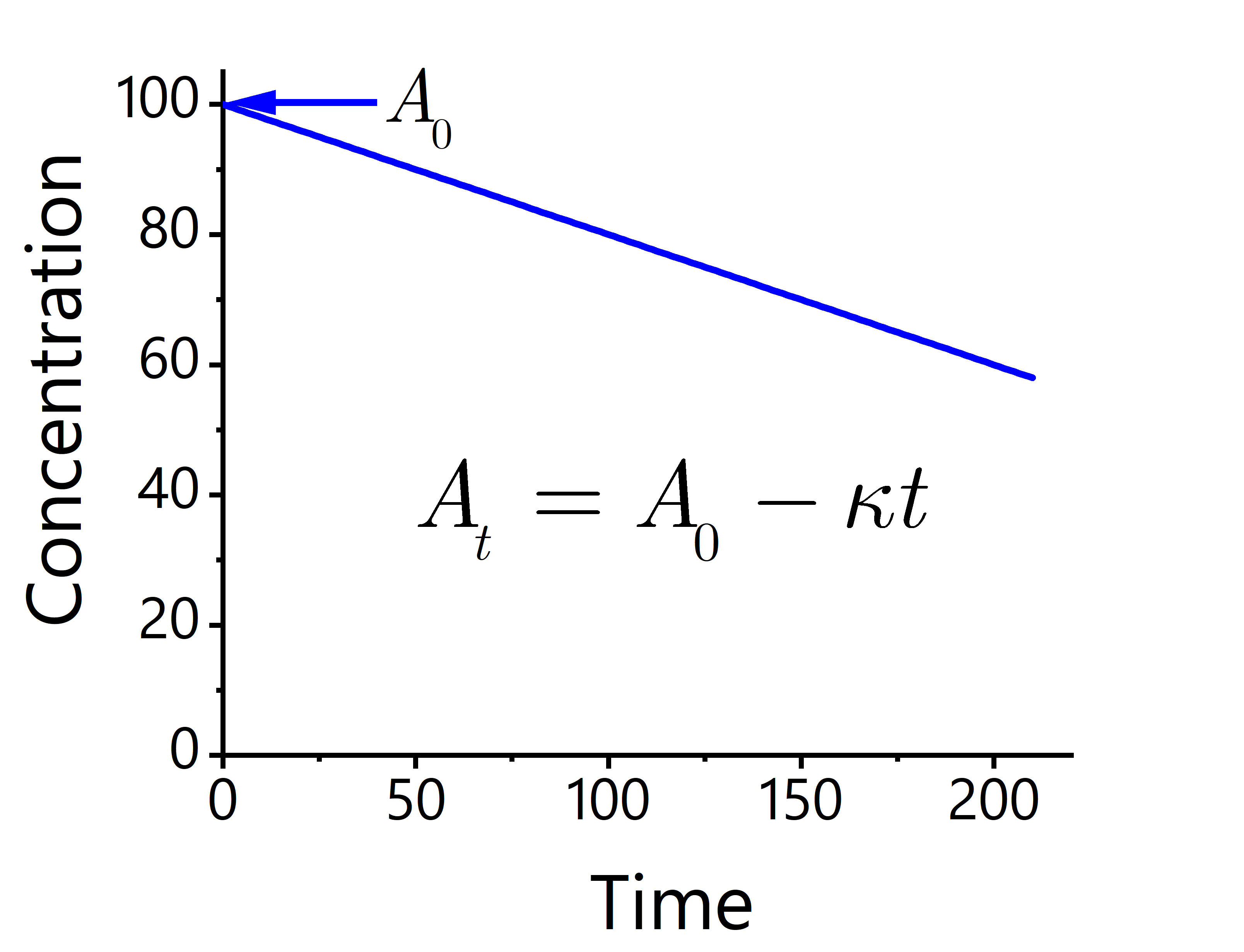
Fig. 49 The graphical trend of a zeroth-order reaction. The change in concentration of reactant and product with time produces a straight line.

Example: Zero-order kinetics

1. Determine the rate constant (\(\kappa\)) of a zero-order reaction if the initial concentration of substance \(A\) is \(\pu{1.5 M}\) and after \(\pu{120 s}\) the concentration of substance \(A\) is \(\pu{0.75 M}\).

In this problem, \([A]_0 = \pu{1.5 M}\), \([A]_t = \pu{0.75 M}\), and \(t= \pu{120 s}\). Using Eq. (65), we can calculate \(\kappa\) as follows:

\[\begin{split}\begin{align*} [A]_t &= [A]_0 - \kappa t\\ (\pu{0.75 M}) &= (\pu{1.5 M}) - \kappa (\pu{120 s})\\ \kappa &= \pu{0.00624 M s−1} \end{align*}\end{split}\]

2. What is the half-life of substance \(A\) (from problem 1) if its original concentration is \(\pu{1.2 M}\)?

In this problem, half-life (\(t_{1/2}\)) refers to the time needed for \([A]_t = 0.5 \cdot [A]_0\). Since \([A]_0 = \pu{1.2 M}\), \([A]_t = \pu{0.6 M}\). We calculated \(\kappa = \pu{0.00624 M s−1}\) in the first problem. Now we can calculate \(t\) using Eq. (65) as follows:

\[\begin{split}\begin{align*} [A]_t &= [A]_0 - \kappa t\\ \pu{0.6 M} &= \pu{1.2 M} - (\pu{0.00624 M s−1}) t_{1/2}\\ \therefore \, t_{1/2} &= \pu{96 s} \end{align*}\end{split}\]

3. If the original concentration of substance \(A\) is reduced to \(\pu{1.0 M}\) in the previous problem, does the half-life decrease, increase, or stay the same? If the half-life changes, what will the new half-life be?

The half-life decreases when the original concentration is reduced. New half-life is \(\pu{80 s}\).

First-order kinetics

A first-order reaction is a reaction that proceeds at a rate that is dependent on the concentration of the reactant. Exponents of all reactants are \(1\) in the expression below:

(66)\[\text{Rate} = \kappa [A][B]\]

For \(A\),

(67)\[\text{Rate} = - \frac{\Delta [A]}{\Delta t} = \kappa_A [A]\]

On integrating,

(68)\[[A]_t = [A]_0 e^{- \kappa_A t}\quad \text{or} \quad \ln \frac{[A]_t}{[A]_0} = - \kappa_A t\]

This equation is represented in Fig. 50.

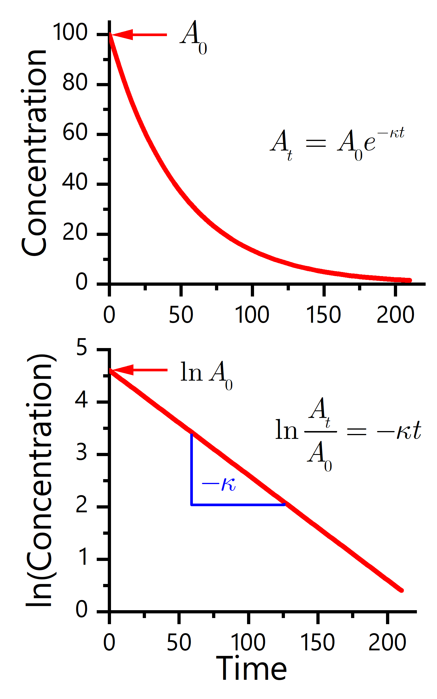
Fig. 50 Graphical trend of a first-order reaction. The expected shapes of the graphs for plots of reactant concentration versus time (top) and the natural logarithm of reactant concentration versus time (bottom) for a first-order reaction.

Example: First-order kinetics

If \(\pu{3.0 g}\) of substance \(B\) decomposes for \(\pu{36 min}\) and the mass of unreacted \(B\) remaining is found to be \(\pu{0.375 g}\), what is the half-life of this reaction if it follows first-order kinetics?

In this problem, \([B]_0 = \pu{3.0 g}\) and \({B]_t = \pu{0.375 g}\), and \(t= \pu{36 min}\). Using Eq. (68), we can calculate \(\kappa\) as follows:

\[\begin{split}\begin{aligned} \ln \frac{[B]_t}{[B]_0} &= - \kappa_B t\\ \ln \frac{\pu{0.375 g}}{\pu{3.0 g}} &= - \kappa_B (\pu{36 min})\\ \therefore \kappa &= \pu{0.0578 min-1} \end{aligned}\end{split}\]

Now that we have determined \(\kappa\) for substance \(B\), we can calculate \(t_{1/2}\) (i.e., when \([B]_t = 0.5 \cdot [B]_0\)) for this substance as follows:

\[\begin{split}\begin{aligned} \ln \frac{[B]_t}{[B]_0} &= - \kappa_B t\\ \ln \frac{(0.5 \cdot [B]_0)}{[B]_0} &= - \kappa_B t_{1/2}\\ \ln 0.5 &= - (\pu{0.0578 min-1}) t_{1/2}\\ \therefore \, t_{1/2} &= \pu{12 min} \end{aligned}\end{split}\]

Example: First-order kinetics

The rate of decomposition of diazomethane is shown in the data below.

Time, \(\pu{s}\)	Conc, \(\pu{ppb}\)
0	284
100	220
150	193
200	170
250	150
300	132

Determine (a) the reaction order and (b) the rate constant for this reaction.

On plotting these data in a \(x-y\) graph resembling Fig. 50 and therefore, this is a first-order reaction. Plot the \(\ln (\text{Conc}) \) vs. \(\pu{Time}\), and the slope of this straight line is the rate constant.